Machine LearningInformation Theory

Interpolation Can Be Harmless

The classical warning about overfitting fused two claims: that a model fits noisy data exactly, and that the fitted noise must damage predictions elsewhere. A Fourier sampling toy separates them — and turns “benign overfitting” into something you can calculate.

In this story

A warning that fused two claims

What was already understood

Fitting noisy training data exactly was long treated as the signature of overfitting: a model that memorizes noise was expected to pay for that memorization on new data.

That warning quietly fuses two different claims: first, that the model fits the noise in its training data exactly; second, that the fitted noise must corrupt its predictions elsewhere. Modern practice pulled the two apart — large neural networks routinely interpolate their training data and still generalize — and the question became why.

Overparameterization is what separates the claims. When there are more feature directions than sample constraints, an interpolating model is obliged to fit the noise, but it retains freedom in where to put it. Generalization then depends on the geometry of that choice, not on the mere fact of interpolation. Our work made that geometry exactly calculable in deliberately tractable linear and Fourier models — first for regression, then for classification, then for many classes, adversarial perturbations, and learning from a weaker teacher's noisy labels.

This question was being attacked from several directions at once. Belkin, Hsu, Ma, and Mandal mapped double descent; Bartlett, Long, Lugosi, and Tsigler characterized benign overfitting through covariance spectra; and Hastie, Montanari, Rosset, and Tibshirani developed precise asymptotics for ridgeless interpolation. Belkin and Hsu later joined us on the classification paper below. What distinguishes the line of work in this story is its instrument: a Fourier sampling model that exposes the mechanism through exact calculation, paired with phase maps that reduce competing effects to comparable exponents.

Overparameterization is undersampling

Our decisive conceptual move, in the ISIT 2019 paper and its expanded JSAIT version, was to turn a high-dimensional puzzle into an elementary problem from signal processing. Take nn regularly spaced samples of a one-dimensional signal, and fit them using more Fourier frequencies than samples. Overparameterization is now literally undersampling.

Sampling theory says exactly what goes wrong — and here, what goes right. Frequencies separated by multiples of the sampling rate, ff and f+knf + kn, are exact aliases: on the training grid they are indistinguishable, taking identical values at every sample. Under the uniform test distribution used in the toy, however, the corresponding Fourier features are exactly orthogonal. The sampled data can be decomposed into discrete Fourier modes, and minimum-2\ell_2-norm interpolation responds to the degeneracy in the most even-handed way possible: it divides the coefficient required for each sampled mode among the frequencies in that mode's alias class.

Parseval's identity then makes the bookkeeping exact. Noise that has been spread over an expanding set of orthogonal directions contributes almost nothing to mean-squared test error — even though every noisy training sample was fit perfectly. The fitted noise is not gone; it has been dissipated into directions that are individually tiny and mutually orthogonal under the test distribution.

Key Insight

Overparameterization is undersampling: extra Fourier frequencies coincide in alias classes on the training grid, yet remain exactly orthogonal under the toy's test-distribution inner product. Aliasing lets the interpolator absorb noise; orthogonality makes the absorbed noise harmless in test error.

Survival and contamination

The same dissipation that disposes of noise can also erase what one wanted to learn. True signal bleeds into aliases just as noise does: the energy of the low-frequency component the data actually came from is likewise split among its high-frequency impostors.

This led us to a pair of complementary bookkeeping quantities. Survival measures how much of the true signal direction remains in the learned predictor. Contamination measures how much the many false directions — the aliases carrying their shares of signal and noise — perturb a prediction at a test point. Harmless interpolation requires both sides of a bargain: enough extra directions to absorb the noise, together with enough inductive preference for the true directions — for instance, feature weights that favor low frequencies — to keep the signal alive while the noise dissipates.

This is why the story cannot be compressed to "noise gets spread across many dimensions." Which directions are aliased with which, and how the interpolator allocates energy among them, is precisely the sampling geometry — and it is that geometry, not high dimensionality alone, that decides whether interpolation is benign or catastrophic.

What this work added

The contribution was not the observation that interpolation of noise can be benign — that was being established concurrently, and in more general settings. What we added was a Fourier model in which overparameterization becomes undersampling, making exact aliasing and exact orthogonality available as instruments for calculating rather than merely describing the effect; and a separation of that calculation into survival and contamination, which turns one question about generalization into two questions with different answers.

The Fourier Ultra Toy

This Fourier construction was part of the work from the beginning, not an illustration we attached afterward. The ISIT 2019 paper already pointed toward the Fourier setting; the full arXiv/JSAIT treatment developed the regular-grid Ultra Toy and its exact alias calculations. Its value is that nothing important is hidden behind a large random matrix: one can watch minimum-norm interpolation allocate every sampled Fourier mode among features that are identical on the training grid and orthogonal under the test-distribution inner product.

The regression side is not confined to one carefully chosen waveform. In the lab below, every smooth target in the menu is supported entirely on the default s=7s=7 favored low-frequency directions. Widen the favored band to see precisely which additional Fourier directions receive the same preference; change the target and the same aliasing mechanism persists. Then switch to the clean 1-1-to-+1+1 step: that deliberately misspecified target is the natural bridge to the classification paper.

Every displayed curve is the exact weighted minimum-2\ell_2-norm Fourier interpolant for the stated finite model. In regression mode, the orange points include one fixed noise realization; in the classification bridge they are clean binary labels. The blue area measures amplitude error, while the red bands mark sign errors.

The regular-grid Fourier Ultra Toy, alias allocation, survival, and contamination come from Harmless Interpolation of Noisy Data in Regression (ISIT 2019; expanded JSAIT 2020 treatment). The n=49n=49, s=7s=7, d=441d=441 presets and λH\lambda_H values reproduce the finite examples in Classification vs regression in overparameterized regimes: Does the loss function matter? (JMLR 2021).

What stays fixed

The training labels and the minimum-norm rule do not change when the evaluation ruler changes. Regression asks whether the amplitude is right; classification asks whether the sign is right. That single change creates the intermediate regime.

Classification is not regression

Exact aliasing and exact orthogonality collapse the mechanism to a calculation simple enough to serve as a conjecture engine. The Fourier "ultra-toy" suggested — and we then established for Gaussian features in the JMLR 2021 paper written with Mikhail Belkin and Daniel Hsu (along with students Vidya Muthukumar, Adhyyan Narang, and Vignesh Subramanian) — that regression and classification obey different thresholds.

Regression needs the predicted value to be right: survival must stay near one and contamination near zero. Classification only needs the surviving signed signal to dominate the contamination — a weakened signal still classifies correctly as long as it outvotes the noise at the test point. The consequence is a genuine intermediate regime in which the very same minimum-norm predictor fails as a regressor while succeeding as a classifier.

There is a second, stranger consequence. With sufficient effective overparameterization, every training point becomes a support vector, and the hard-margin SVM — trained on a completely different loss — coincides exactly with the minimum-norm least-squares interpolator. In these regimes, the choice of training loss can matter far less than the geometry both losses inherit.

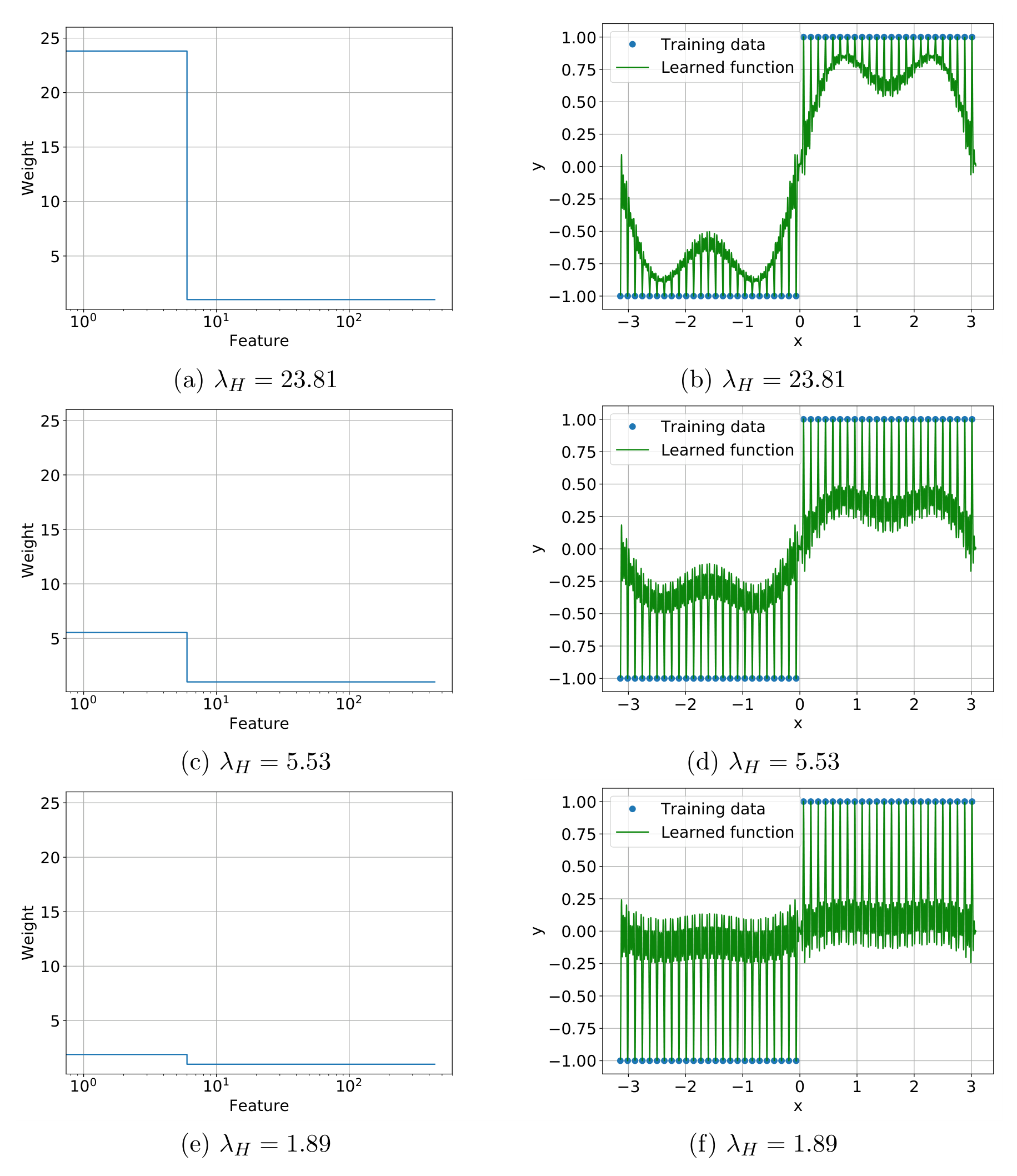
Six panels in three rows showing low-frequency feature weights and minimum-norm interpolation of binary step labels: accurate amplitude, attenuated but mostly correct sign, and severe signal loss.

Three finite regimes in the Fourier Ultra Toy, controlled by λH\lambda_H — the weight placed on the favored low-frequency features, plotted in the left column. Top: the learned function retains enough amplitude for regression and classification. Middle: its amplitude is badly attenuated, but its sign remains right almost everywhere. Bottom: even the sign is lost in this displayed finite example. The JMLR paper proves the corresponding three-way separation for its Gaussian model; it explicitly leaves the matching asymptotic Fourier lower bound in the third regime open.

Why the thresholds differ

A regressor must recover the amplitude of the true signal; a classifier only needs the weakened surviving signal to outvote the contamination. Between those two thresholds lives a regime where the same predictor is a failed regressor and a working classifier.

Turning mechanisms into phase maps

Our second major tool was a deliberately physics-style use of asymptotics. Instead of sending sample size and dimension to infinity along one fixed aspect ratio, we write each structural quantity as a power of the number of training points nn: the number of features scales as npn^p, the number of favored directions as nrn^r, the strength of the favoring enters through an exponent qq, and — in the later work — the number of classes grows as ntn^t.

Every competing mechanism now owns an exponent, and comparing exponents turns complicated non-asymptotic bounds into linear boundaries between regions: a phase map. One region where regression and classification both succeed; one where classification alone succeeds; one where nothing does. The maps did not merely summarize finished theorems — they organized the search for theorems, separating effects that tangle together at any single problem size and identifying which result should be true in each region. We then progressively filled in these maps across the multiclass papers: NeurIPS 2022 established achievable regions, ISIT 2023 supplied a matching converse, and the NeurIPS 2023 paper sharpened the lower bounds into strong converses that pin the boundaries exactly.

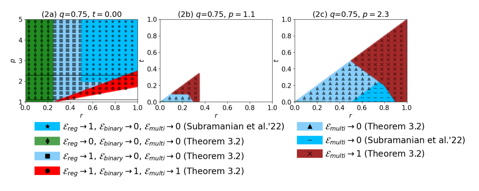
Three phase-map panels showing regions of the exponent space where regression, binary classification, and multiclass classification succeed or fail, with a legend identifying each region.

The mature phase-map view. Every axis is a scaling exponent, with the favored-direction exponent rr running horizontally throughout: the left panel varies the feature exponent pp against rr at a fixed number of classes, while the middle and right panels vary the class-count exponent tt against rr at two fixed values of pp. Each colored region records which tasks succeed — regression error Ereg\mathcal{E}_{reg}, binary classification error Ebinary\mathcal{E}_{binary}, and multiclass error Emulti\mathcal{E}_{multi} tending to 00 or 11. The strong converses turn the boundaries from conjectured lines into exact ones.

The method, not just the map

Writing every structural quantity as a power of nn gives each competing mechanism its own exponent, and turns the comparison of mechanisms into a comparison of numbers. That was a method of discovery rather than a way of summarizing finished work: the maps told us which theorem ought to be true in each region before we could prove it.

Ridge regression, seen wider

A smaller observation we made in the JSAIT regression paper deserves its own moment, because it makes the regularizing role of extra features concrete. The familiar "pseudo-observation" view of ridge regression makes the data matrix taller: append fake training examples with zero targets, and the ridge solution appears.

The alternative view makes it wider: append one sample-specific feature per training point — a scaled identity block — and solve an ordinary minimum-norm interpolation problem. Those private features can absorb each training point's residual, but they contribute nothing at a test point, where they are never active. The two constructions impose exactly the same spectral shift, so ridge regression is minimum-norm interpolation with extra feature directions. Additional dimensions, used this way, do not enlarge a model so much as regularize it — the same moral the aliasing story tells, in matrix form.

Where the mechanism leads

Once survival, contamination, and the phase-map method exist, they travel.

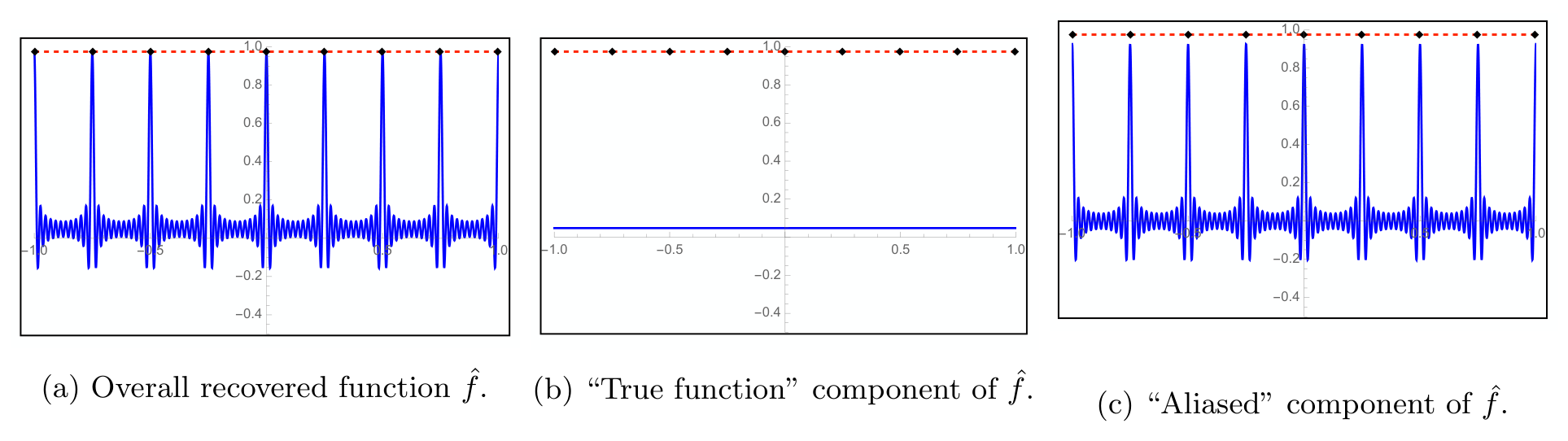
Adversarial examples. The aliased component is not spread uniformly in space but concentrated in sharp, Gibbs-like spikes near the training samples. Contamination can be small on average — so ordinary classification succeeds — while being locally enormous, so that tiny input perturbations near training data flip predictions. Low test error and proliferating adversarial failures are not in tension; in this model they are the same geometry read at two different scales.

Three panels showing a minimum-norm interpolation of a constant function: the overall recovered function with spikes at training points, the small constant surviving component, and the aliased component concentrated near the samples.

The spatial structure hidden by an average test-error number. A minimum-2\ell_2-norm Fourier interpolator decomposes into an attenuated surviving component and an aliased component concentrated in sharp spikes near the training samples — precisely where small perturbations can become consequential.

Many classes. Multiclass classification asks the surviving signal to win more comparisons with less margin. We extended the phase maps to a growing number of classes, located the new boundaries, and — in the NeurIPS 2023 paper — proved matching lower bounds and strong converses, so the map's frontiers are exact rather than conjectured.

Weak-to-strong generalization. A Fourier counterpart makes the connection vivid. If a weak alias is present in the teacher model, then giving the student more pseudo-labeled samples puts that alias into the samples themselves. The student could learn it. But the inductive bias does not preserve every teacher-side direction equally: the weak alias does not survive strongly enough to be learned, while the true direction does. In the formal Gaussian-feature model, the same competition is measured through survival and contamination. The student can fit the imperfect supervision exactly without inheriting every error that produced it, and can therefore generalize beyond the teacher.

The through-line of the whole story is a method as much as a result: build the smallest world in which a mechanism operates exactly, calculate it there, and let the exponents say where each phenomenon begins and ends. The Fourier toy and the phase maps remain live instruments for us, and this arc is still being extended.
Scope and caveats

These are linear and Fourier toy models by design. The claim is not that they explain every neural network; it is that phenomena often bundled together as "overfitting" can be separated, calculated, and proved to have different phase boundaries.

The papers

Our ISIT 2019 paper introduced the harmless-interpolation problem and already pointed toward the Fourier setting. Its expanded arXiv/JSAIT version developed the Fourier Ultra Toy, exact alias calculations, survival and contamination, and the wide-feature view of ridge. The JMLR 2021 paper used that Ultra Toy to conjecture the classification/regression separation and support-vector proliferation, then established the corresponding results in the Gaussian model. The 2021 signal-processing paper made the mechanism spatially visible, including its adversarial consequences. The NeurIPS 2022 and ISIT 2023 papers opened up the multiclass phase maps, the NeurIPS 2023 paper closed them with precise asymptotics and strong converses, and the ICLR 2025 paper carried benign overfitting to weak-to-strong generalization.

Related Papers
2019IEEE Interational Symposium on Information Theory
2020IEEE Journal on Selected Areas in Information Theory
2021Journal of Machine Learning Research
2021ICML Workshop on Overparameterization: Pitfalls & Opportunities
202236th Conference on Neural Information Processing Systems
2023IEEE International Symposium on Information Theory
202337th Conference on Neural Information Processing Systems (NeurIPS)
2025International Conference on Learning Representations (ICLR), Apr, 2025